
Price volume mix analysis: the complete guide
How to break down a revenue or margin variance into volume, price and mix effects, with no double counting and no unexplained residual. Formulas, the classic trap, and a method to build an analysis your finance leader…
Revenue moved. Margin did too. The first question you get is "why", and "we sold more" is never enough. Did you sell more units (volume effect)? Did the average selling price change (price effect)? Or did you simply sell a different mix of products, customers or channels, with volumes and prices unchanged (mix effect)? These are three different questions, with three different operational answers, and most analyses built by hand in Excel blend them without anyone noticing.
This guide walks through the full method: the formulas, the double-counting trap that invalidates most homemade models, an end-to-end numbered example, and how to rerun the calculation on a test dataset in Datama.
What is price volume mix analysis?
Price volume mix analysis (sometimes called PVM) breaks down the change in an indicator (revenue or margin) between two periods or two perimeters into three families of effects:
- Volume effect: how much of the variance comes from the number of units sold, all else equal?
- Price effect: how much comes from the average selling price?
- Mix effect: how much comes from a change in the composition of sales (more of product A, less of product B, a channel gaining weight), even if nobody changed a list price or a commercial policy?
The third effect is the one almost nobody isolates cleanly. A falling average price can mean two opposite things: either you really cut prices, or you simply sold more of SKUs that were already cheaper. The decision you take is not the same in both cases, and without a decomposition you cannot tell them apart.
Why the mix effect is harder to isolate than it looks
An average price or an average cost is a weighted average computed across your whole range. As soon as the weights change (more volume on one segment, less on another), the average moves mechanically, without any pricing decision having been taken. That shift in weighting is the mix effect, and it lives inside your price and cost metrics, not next to them.
We unpacked this mechanism in depth, with a line-by-line example, in our case study on the mix effect of weather: total revenue rises slightly, but the sales mix shifts towards a cheaper product, and the average price falls even though nobody changed a tariff. The same phenomenon shows up on a margin, an acquisition cost, or any metric built as an average.
The base formula
For revenue, the two-factor decomposition is:
Revenue = Volume × Average price
From there, the total variance between period 0 and period 1 splits into two top-level effects:
- Volume effect = (Volume₁ - Volume₀) × Price₀
- Price effect = Volume₁ × (Price₁ - Price₀)
Added together, these two effects reconstitute the total revenue variance exactly. So far, no issue: it is a two-term decomposition, so it cannot leave a residual.
The problem starts when you want to go further and, inside the price effect, separate a genuine tariff change from a change in composition. That is where the third effect, the mix effect, appears, and where most Excel models break.
Trap number one: double counting
As soon as you break a variance into more than two effects (volume, price, mix, cost…), there are infinitely many mathematically valid ways to allocate the movement between them, and most of them either leave a residual or count the same movement twice.
The most common error: compute the volume effect with the starting-period price, then compute the price effect with the arriving-period volume (or the other way around). Each effect looks correct in isolation, but their sum does not reconstitute the total variance exactly. The leftover gap, often labelled "cross effect" or "mix effect" by default, is actually a calculation artefact: nobody can explain it to an executive committee because it corresponds to nothing operational.
We documented the same trap for margin, with the three symptoms that give a poorly built model away (the numbers do not add up, mix and true price are blended, the model breaks as soon as you add a dimension), in Stop getting your margin analysis wrong. The cause is the same on a classic price volume mix: without an explicit, consistent allocation method, the decomposition is not reliable, even if the spreadsheet looks tidy.
What a sound decomposition must guarantee:
- Effects are additive: their sum reconstitutes the total variance exactly, to the last euro.
- Effects are orthogonal: no effect contains part of another effect's explanation.
- The result does not depend on an arbitrary choice of "which effect we compute first".
Decomposing cleanly: volume, price, mix
Once the volume effect is isolated on the base formula, the price effect itself splits into two components, by analysing the composition inside the average price:
- Mix effect: variance due to a shift in weight between segments (more volume on high-price SKUs, or the reverse), with each segment's unit price unchanged.
- True price effect (or rate effect): variance due to a genuine tariff change inside each segment, with composition unchanged.
In practice, that means going down to the segment (product, range, customer, channel, depending on your business) rather than reasoning on a global average price, then recomposing the two effects with a consistent allocation method from one end of the calculation to the other. The arithmetic is mechanical, but it quickly becomes unmanageable by hand once you have more than a handful of segments or you want to rerun it every month.
A numbered example
Take a company that sells two product ranges, A and B. Between month M and month M+1:
| Month M | Month M+1 | |
|---|---|---|
| Product A volume | 800 units at 25 € | 600 units at 25 € |
| Product B volume | 200 units at 10 € | 500 units at 10 € |
| Total revenue | 22,000 € | 20,000 € |
| Average price | 22 € | 18.18 € |
No price has changed. Yet revenue is down 2,000 € and the average price has dropped by nearly 4 €. A quick reading of the average price ("our prices are deteriorating") would be wrong: it is the sales mix that has shifted towards product B, which is cheaper, and whose weight has gone from 20% to 45% of units sold.
A clean decomposition isolates:
- Volume effect: +2,200 €. Total volume grows by 10% (1,000 → 1,100 units), valued at the starting average price of 22 €.
- Mix effect: -4,200 €. The shift towards product B mechanically pulls the average price, and therefore revenue, down.
- True price effect: 0 €; no tariff has moved.
The three effects add up exactly to the 2,000 € drop. Sales grow in volume, but the mix wipes out that gain and more.
Without that decomposition, the commercial team would be left justifying a "price cut" that never happened, and looking for an explanation on the wrong side.
How Datama Compare automates this calculation
Datama Compare applies this decomposition method (the "market equation") to any indicator expressed as a combination of factors, with no manual recalculation:
- Guaranteed additive decomposition: volume, price and mix effects reconstitute the total variance exactly, with no residual.
- Automatic mix / performance split: for every dimension in your dataset (product, customer, region, channel…), Datama distinguishes what comes from a change in composition from what comes from a rate change inside each segment.
- Ranking by explanatory dimensions: rather than listing every available dimension, Datama ranks them with an interest score that shows which one actually explains the observed variance, not merely which one has the most rows.
- Contribution by segment: down to which product, customer or area is pulling the effect up or down, and by how much.
The result is read as a Waterfall (cascade chart): each effect stacks visually between the starting point and the end point, and can be read in under 30 seconds. You can go further by building your own market equation; we walked through the method in How to build my business metric relation.
For a margin rather than revenue, the equation simply extends (Margin = Volume × (Price - Cost per unit)), and each extra term adds an effect to the Waterfall without changing the method. The full detail is in Stop getting your margin analysis wrong.
The template: your first analysis in 15 minutes
The fastest path is not to rebuild the calculation in Excel, but to reread it on a test dataset, then run Datama Compare on it.
1. Open the test dataset. Use the price volume mix demo dataset: an aggregated table with a comparison dimension (the month), explanatory dimensions (country, channel, product) and summable metrics (units sold, revenue, margin). That is the format Datama expects: no precomputed ratios. Datama calculates them.
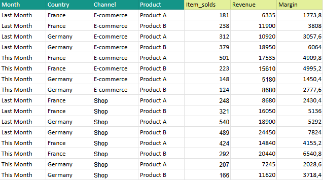
2. Launch Datama. Connect this dataset in Datama Compare. The equation used is of the form Margin = Volume × Average price × Margin rate. The waterfall reconstitutes the margin variance exactly, with no residual.
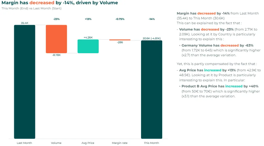
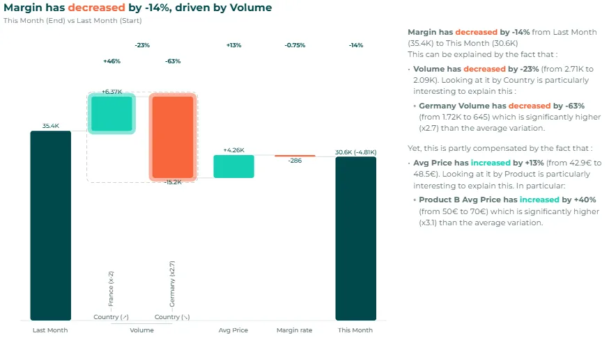
The volume effect is the first column: it is the quantity of items sold. Here, volume is down, mainly in Germany.
The second column is average price (revenue / quantity). Once opened, it splits into two effects: performance, which is the true price effect, and mix, which is the change in weight of product types in sales.
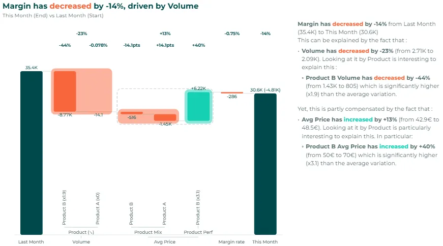
Here, on product B, a rise in production cost reduced sales volumes, especially in Germany (as seen in the previous point). That drop has a double effect on average price: a negative mix effect (product B, which used to sell at a higher price, weighs less, and the reverse for product A) and a positive price effect, driven by the rise in product B's net price.
The margin rate has barely moved: the slight variance comes from the mix between products A and B, which do not have quite the same margin rate.
Datama Compare is available where your data already lives: Google Sheets, Excel, Skill (Claude, ChatGPT) or your usual visualisation tools (Power BI, Tableau, Looker Studio, Qlik).
Who this analysis is for
- Financial controllers who have to justify a revenue or margin gap in the monthly pack.
- Category managers and pricing leads who need to know whether a change in average price comes from a genuine tariff decision or from a composition effect.
- FP&A teams who prepare variance explanations for an executive committee and cannot afford an unexplained residual.
Frequently asked questions
What is the difference between the price effect and the mix effect? The price effect measures price changes within each product or segment. The mix effect measures the change in the composition of sales at unchanged prices: selling more of cheaper products lowers the average price even if no price list moved.
Does a price volume mix analysis leave a residual? Not if the decomposition is additive. A two-factor split (volume × price) never leaves one. Beyond two effects, most homemade models either leave a residual or count the same movement twice, which is the trap described above.
Does PVM analysis work for margin as well as revenue? Yes. For margin, the equation adds the cost side: Margin = Volume × (Price − Cost per unit). See stop getting your margin analysis wrong.
What data do I need? Two periods (or actual and budget) at the same grain, for example month × product × customer, with additive metrics: units and revenue, plus cost for a margin analysis. No pre-computed averages: the ratios are calculated from the totals.
Can I run a price volume mix analysis in Power BI or Excel? Yes. Datama runs it natively in Power BI, Excel, Tableau and the other integrations.
In short
A revenue or margin variance never has a single cause. It always decomposes into volume, price and mix, and until those three effects are isolated cleanly, without double counting, every explanation remains a hypothesis. The method described here (additive formula, mix / performance split, numbered example) works by hand for a simple case; Datama Compare automates it as soon as the number of segments or the frequency of the analysis makes a manual calculation untenable.
→ Learn more about the solution: datama.io
Related articles
- Articles
Variance analysis: sales, revenue or margin bridge?
Variance analysis does not stop at the variance: it explains it. Sales, revenue or margin bridge, which method to use depending on the question asked.
- Articles
Stop getting your margin analysis wrong
How finance teams are finally fixing it in Excel. Every CFO has been there. The monthly close lands, margin is down 1.2 points, and the CEO is already asking: why? The answer is somewhere in a sprawling Excel workbook…
- Articles
Mix effect of weather on sales revenue
Have you ever considered how weather might influence a company’s performance? To what extent can it make an impact, and how? Perhaps you’re aware that weather affects KPIs, but not in enough detail to explain its infl…
Want the why behind your own numbers?
Try Datama free, or book a 30 minute demo with the team.